Density estimation
A trajectory gives you where every particle is. What you usually want to look at is where the particles are, as a smooth field over the surface rather than a cloud of dots. wanderwalk ships two kernel density estimators for that, one per geometry, plus a histogram for the hyperbolic boundary.
Both estimators take the final positions and a mesh you supply, and return density values on that mesh, normalized so the maximum is 1. They are built for plotting, not for integration.
sphere_kde
The kernel measures closeness with the dot product between a particle and a
mesh point. On the unit sphere both have norm 1, so a larger dot product
means a smaller geodesic distance, and the weight exp(k * dot) falls off
as you move away from a particle.
You build the mesh yourself, which means you control the resolution:
import numpy as np
import wanderwalk as ww

np.random.seed(0)
trajectory = ww.sphere_simulator(T=60, N=3000, dt=0.01, noise_type="isotropic")

u, v = np.mgrid[0:2 * np.pi:120j, 0:np.pi:60j]
x = np.cos(u) * np.sin(v)
y = np.sin(u) * np.sin(v)
z = np.cos(v)

density = ww.sphere_kde(trajectory[-1], x, y, z, N=3000)

print("density shape:", density.shape)
print("range:", round(float(density.min()), 6), "to", float(density.max()))
The output has the same shape as the mesh arrays, so it drops straight into
plot_surface as face colors:
import matplotlib.pyplot as plt
import numpy as np
import wanderwalk as ww

np.random.seed(0)
trajectory = ww.sphere_simulator(T=60, N=3000, dt=0.01, noise_type="isotropic")

u, v = np.mgrid[0:2 * np.pi:120j, 0:np.pi:60j]
x, y, z = np.cos(u) * np.sin(v), np.sin(u) * np.sin(v), np.cos(v)
density = ww.sphere_kde(trajectory[-1], x, y, z, N=3000)

fig = plt.figure(figsize=(5, 5))
ax = fig.add_subplot(projection="3d")
ax.plot_surface(x, y, z, facecolors=plt.cm.magma(density), linewidth=0, shade=False)
ax.set_box_aspect([1, 1, 1])
ax.set_axis_off()
plt.show()
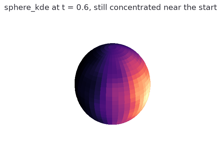
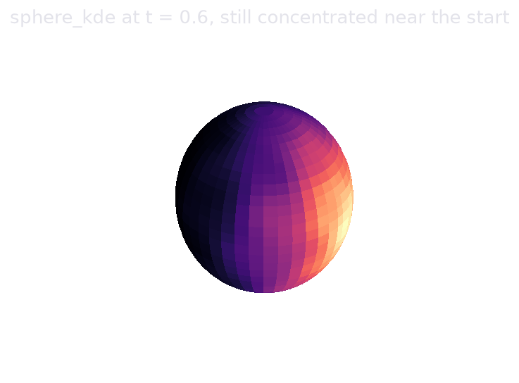
At t = 0.6 the particles have not gone far, so the hot spot sits right on
the starting point (1, 0, 0):
import numpy as np
import wanderwalk as ww

np.random.seed(0)
trajectory = ww.sphere_simulator(T=60, N=3000, dt=0.01, noise_type="isotropic")

u, v = np.mgrid[0:2 * np.pi:120j, 0:np.pi:60j]
x, y, z = np.cos(u) * np.sin(v), np.sin(u) * np.sin(v), np.cos(v)
density = ww.sphere_kde(trajectory[-1], x, y, z, N=3000)

hottest = np.unravel_index(np.argmax(density), density.shape)
print("hottest mesh point:", np.round([x[hottest], y[hottest], z[hottest]], 4))
disk_kde
The hyperbolic version cannot use the Euclidean distance in the picture,
because the picture is distorted. Two points that look equally far apart near
the rim and near the center are not. So disk_kde computes the exact
hyperbolic geodesic distance between every particle and every mesh point,
and weights with exp(-k * d^2).
Mesh points outside the unit disk are not part of the space at all, so they
come back as NaN:
import numpy as np
import wanderwalk as ww

np.random.seed(0)
trajectory = ww.hyperbolic_simulator(T=300, N=3000, dt=0.01)

grid = np.linspace(-1.2, 1.2, 200)
x_mesh, y_mesh = np.meshgrid(grid, grid)
density = ww.disk_kde(trajectory[-1], x_mesh, y_mesh, k=40)

inside = (x_mesh ** 2 + y_mesh ** 2) < 1.0
print("mesh points inside the disk:", int(inside.sum()), "of", density.size)
print("NaN entries:", int(np.isnan(density).sum()))
NaN is deliberate. Matplotlib leaves those cells blank, so the disk comes
out as a disk rather than a square with a circle drawn on it. Use
np.nanmax and friends when you need summary statistics.
import matplotlib.pyplot as plt
import numpy as np
import wanderwalk as ww

np.random.seed(0)
trajectory = ww.hyperbolic_simulator(T=300, N=3000, dt=0.01)

grid = np.linspace(-0.99, 0.99, 300)
x_mesh, y_mesh = np.meshgrid(grid, grid)
density = ww.disk_kde(trajectory[-1], x_mesh, y_mesh, k=40)

fig, ax = plt.subplots(figsize=(5, 5))
ax.pcolormesh(x_mesh, y_mesh, density, cmap="magma", shading="auto")
ax.add_patch(plt.Circle((0, 0), 1.0, fill=False, color="black"))
ax.set_aspect("equal")
ax.set_axis_off()
plt.show()
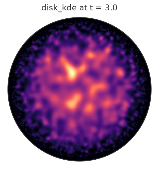
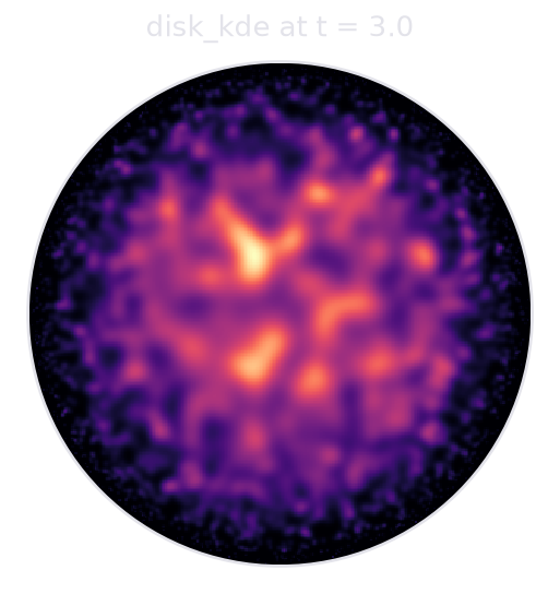
This is a picture, not a probability density
Both estimators normalize so the peak is 1, and neither divides by the Riemannian area element. They do not integrate to 1 over the surface, and for the Poincare disk there is no stationary density to converge to anyway, since the motion is transient. If you want a density that can be compared against theory, see the heat kernel tutorial, which does the area-element normalization properly.
Choosing k
k is the concentration parameter. Large k makes each particle contribute
a tight spike, so the estimate is spiky and noisy. Small k smears
everything together, so the estimate is smooth and washed out.
Both functions default k to sqrt(N) when you pass N, and to 20 when you
pass neither:
That default scales sensibly: more particles support a sharper kernel. The two arguments interact in a way worth stating plainly:
| You pass | What happens |
|---|---|
k=40 |
k is 40. N is ignored. |
N=3000 |
k becomes sqrt(3000), about 54.8. |
| neither | k is 20. |
| both | k wins; N is ignored. |
Start with the default, then adjust if the picture is too grainy (lower k)
or too flat (raise k).
k means different things in the two functions
sphere_kde weights with exp(k * dot_product) and disk_kde with
exp(-k * distance^2). Both get sharper as k grows, but a given
numerical value does not produce the same width on both surfaces. Tune
them separately.
boundary_angle_histogram
The third tool is not a density at all. On the hyperbolic plane the interesting limit lives on the boundary circle, so what you want is the distribution of angles among particles that have travelled far out:
import numpy as np
import wanderwalk as ww

np.random.seed(0)
trajectory = ww.hyperbolic_simulator(T=1500, N=2000, dt=0.01)

counts, edges = ww.boundary_angle_histogram(trajectory[-1], radius_threshold=0.9, bins=8)
print("counts:", counts)
print("edges span:", round(float(edges[0]), 4), "to", round(float(edges[-1]), 4))
The return is exactly what np.histogram returns, a counts array and a bin
edges array one longer. The hyperbolic tutorial uses it
to test uniformity on the boundary.
Two things to watch:
- It returns
(None, None), not empty arrays, when no particle has reachedradius_threshold. radius_thresholdis a Euclidean radius in the picture, not a hyperbolic distance. A threshold of 0.9 corresponds to a geodesic distance of about 2.9 from the origin.
What next
- The heat kernel, for a density estimate that is properly normalized and can be checked against an exact formula.
- The visualization API reference.