Brownian motion on the torus
The torus is the surface of a donut. Unlike the sphere it is not homogeneous: the outer rim bulges outward and the inner rim curves back on itself, so the two are not interchangeable. That asymmetry is visible in the simulation, and it is what makes the torus more interesting than a first glance suggests.
The two radii
ww.torus_simulator needs two extra arguments the sphere did not:
| Argument | Meaning |
|---|---|
R |
Major radius, from the center of the hole to the center of the tube. |
r |
Minor radius, the radius of the tube itself. |
import numpy as np
import wanderwalk as ww

np.random.seed(0)
trajectory = ww.torus_simulator(T=200, N=500, dt=0.01, R=3.0, r=1.0)

print(trajectory.shape)
Like the sphere, the torus is a surface sitting inside three-dimensional
space, so positions are points in R^3 and the trajectory is (T, N, 3).
Every particle stays between R - r and R + r from the central axis:
import numpy as np
import wanderwalk as ww

np.random.seed(0)
trajectory = ww.torus_simulator(T=3000, N=5000, dt=0.01, R=3.0, r=1.0)

distance_from_axis = np.linalg.norm(trajectory[-1][:, :2], axis=1)
print(f"min {distance_from_axis.min():.4f}, max {distance_from_axis.max():.4f}")
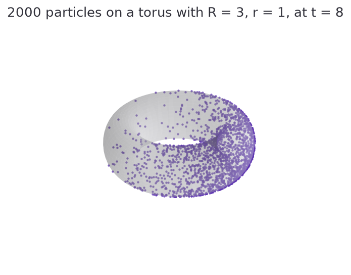
Angles are easier to reason about than coordinates
A point on the torus is naturally described by two angles rather than three coordinates:
- the toroidal angle
u, going the long way around the central hole, - the poloidal angle
v, going the short way around the tube.
ww.Torus converts between the two representations. parametrize goes from
angles to Cartesian coordinates, and angles_from_points goes back for a
whole array at once:
import numpy as np
import wanderwalk as ww

torus = ww.Torus(R=3.0, r=1.0)

point = torus.parametrize(0.0, 0.0)      # u = 0, v = 0
print("outer equator point:", point)

u, v = torus.angles_from_points(np.array([point]))
print("recovered angles:", u[0], v[0])
v = 0 is the outer equator, the circle furthest from the central axis.
v = pi is the inner equator, the circle running through the hole.
The particles do not spread evenly
On the sphere, the long-run distribution is uniform over the surface. That is
also true on the torus, but "uniform over the surface" does not mean "uniform
in the angles". The tube is fatter on the outside than on the inside, so a
band of poloidal angles near v = 0 covers more area than the same band near
v = pi.
Concretely, the area element of the torus is proportional to R + r cos(v),
so the long-run density of the poloidal angle is
which is largest at v = 0 and smallest at v = pi. The simulation
reproduces it:
import numpy as np
import wanderwalk as ww

R, r = 3.0, 1.0
torus = ww.Torus(R, r)

np.random.seed(0)
trajectory = ww.torus_simulator(T=3000, N=5000, dt=0.01, R=R, r=r)
_, poloidal = torus.angles_from_points(trajectory[-1])

counts, edges = np.histogram(poloidal, bins=6, range=(-np.pi, np.pi), density=True)
centers = 0.5 * (edges[1:] + edges[:-1])

for center, simulated in zip(centers, counts):
    theory = (R + r * np.cos(center)) / (2 * np.pi * R)
    print(f"v = {center:+.2f}   simulated {simulated:.4f}   theory {theory:.4f}")
v = -2.62   simulated 0.1245   theory 0.1132
v = -1.57   simulated 0.1646   theory 0.1592
v = -0.52   simulated 0.1898   theory 0.2051
v = +0.52   simulated 0.2057   theory 0.2051
v = +1.57   simulated 0.1581   theory 0.1592
v = +2.62   simulated 0.1121   theory 0.1132
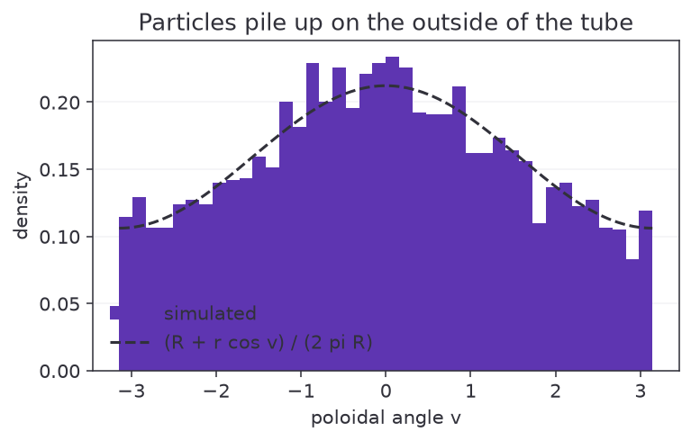
Particles are about twice as likely to be found on the outside of the tube as
on the inside, which is exactly the ratio (R + r) / (R - r) = 4 / 2 of the
two circumferences.
The two directions equilibrate at different speeds
The poloidal angle settles quickly, because the loop around the tube is
short: its circumference is 2 pi r, about 6.3 here. The toroidal angle
takes far longer, because the loop around the hole has circumference
2 pi R, about 18.8, and diffusion covers distance like sqrt(t). At
t = 30 the poloidal histogram above has converged while the toroidal
one is still visibly lumpy around the starting angle. If you want a
genuinely well-mixed torus, run for longer than you would need on a
sphere of comparable size.
Anisotropic noise and the two equators
With noise_type="anisotropic", motion is restricted to e_u, the tangent
direction that goes around the central axis. You might expect the poloidal
angle to be frozen, since the particle only ever moves the long way around.
It is not, and the reason is worth understanding.
import numpy as np
import wanderwalk as ww

R, r = 3.0, 1.0
torus = ww.Torus(R, r)

for v0 in (0.0, 1.0, 2.0, 3.0, np.pi):
    start = torus.parametrize(0.0, v0)
    np.random.seed(0)
    trajectory = ww.torus_simulator(
        T=1000, N=300, dt=0.01, R=R, r=r,
        noise_type="anisotropic", starting_point=start,
    )
    _, poloidal = torus.angles_from_points(trajectory[-1])
    print(f"started at v = {v0:.4f}   after t = 10, mean v = {poloidal.mean():+.5f}")
started at v = 0.0000   after t = 10, mean v = +0.00000
started at v = 1.0000   after t = 10, mean v = +0.29484
started at v = 2.0000   after t = 10, mean v = +0.65355
started at v = 3.0000   after t = 10, mean v = +1.91169
started at v = 3.1416   after t = 10, mean v = +3.14159
The two equators, v = 0 and v = pi, are exactly fixed: particles started
there stay there to the last decimal place. Everywhere else the poloidal
angle drifts toward the outer equator.
That is not a numerical artifact. Shrinking dt by two orders of magnitude
changes the answer by less than 10^-3, so it survives the continuum limit.
The cause is geometric: a circle of constant v is a closed geodesic of the
torus only at v = 0 and v = pi. At any other v, the circle bends within
the surface, and diffusing along a curved path produces a drift along its
geodesic curvature. The outer equator attracts, and the inner equator, though
fixed, repels.
A useful contrast with the sphere
On the sphere, anisotropic noise confines particles to a great circle exactly and forever, because great circles are geodesics. The torus shows what happens when the direction field you pick is not geodesic: the particles slide off it.
Choosing where to start
starting_point takes a point in R^3 on the torus, which is most easily
produced with parametrize:
import numpy as np
import wanderwalk as ww

torus = ww.Torus(R=3.0, r=1.0)
inner_equator = torus.parametrize(0.0, np.pi)

np.random.seed(0)
trajectory = ww.torus_simulator(
    T=100, N=200, dt=0.01, R=3.0, r=1.0, starting_point=inner_equator,
)

print("start:", np.round(inner_equator, 4))
print("distance from axis at t = 1:", round(float(np.linalg.norm(trajectory[-1][0, :2])), 4))
The particle starts on the inner equator, 2 units from the axis, and has begun working its way outward toward the fatter part of the tube.
What next
- The hyperbolic plane, the one surface here where the particles never settle down.
- Driving the manifolds directly, which covers
Torus.project_to_tangent,normal_vector, and stepping one particle at a time.