The hyperbolic plane
The hyperbolic plane is the surface where the behavior is least like the flat case, and where wanderwalk's API deviates most from the other two manifolds. It has constant negative curvature. Brownian motion on it is transient: rather than equilibrating, a particle runs off to infinity and never comes back.
Why the trajectory has only two coordinates
The sphere and the torus are surfaces sitting inside R^3, so a point on them is a vector in R^3 that happens to satisfy a constraint. The hyperbolic plane admits no such description. Hilbert's theorem says it has no isometric embedding into three-dimensional space, so there is no surface in R^3 whose intrinsic geometry is hyperbolic.
wanderwalk therefore represents it intrinsically, in the Poincare disk model:
points are genuine 2D vectors in the open unit disk, and the trajectory has
shape (T, N, 2).
import numpy as np
import wanderwalk as ww

np.random.seed(0)
trajectory = ww.hyperbolic_simulator(T=1500, N=2000, dt=0.01)

print(trajectory.shape)
There is also no noise_type argument. The anisotropic variant is defined by
picking a distinguished tangent direction out of the ambient embedding, and
there is no ambient space here to pick it from.
Euclidean distance is not hyperbolic distance
The unit disk is only a chart. The hyperbolic metric stretches it, by a
factor called the conformal factor, lambda(x) = 2 / (1 - |x|^2). Near the
center one unit of the picture is about half a unit of real distance; near
the rim, one unit of the picture is an enormous distance.
import numpy as np
import wanderwalk as ww

disk = ww.PoincareDisk()

for radius in (0.0, 0.6, 0.99):
    point = np.array([radius, 0.0])
    print(
        f"|x| = {radius:<5} "
        f"conformal factor {disk.conformal_factor(point):>10.4f}   "
        f"geodesic distance {disk.geodesic_distance_from_origin(point):.4f}"
    )
|x| = 0.0   conformal factor     2.0000   geodesic distance 0.0000
|x| = 0.6   conformal factor     3.1250   geodesic distance 1.3863
|x| = 0.99  conformal factor   100.5025   geodesic distance 5.2933
The boundary circle |x| = 1 is infinitely far away. That is why a particle
can approach it forever without ever arriving, and why |x| is a misleading
way to measure how far a particle has travelled. Use
geodesic_distance_from_origin instead, which computes 2 arctanh(|x|).
The most common mistake
Reading |x| as a distance makes the motion look like it is slowing to a
halt near the rim. It is not. The particle is covering more and more
hyperbolic ground for less and less visible movement.
Transience: watch them leave
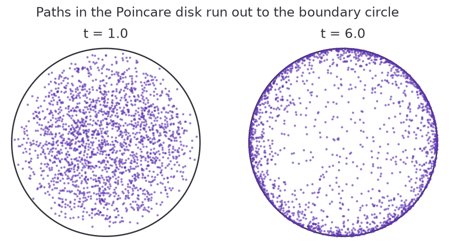
By t = 6 almost every particle is pressed against the rim. The two measures
of how far out a particle has got tell very different stories:
import numpy as np
import wanderwalk as ww

disk = ww.PoincareDisk()

np.random.seed(0)
trajectory = ww.hyperbolic_simulator(T=1500, N=2000, dt=0.01)

for step in (99, 299, 699, 1499):
    positions = trajectory[step]
    t = (step + 1) * 0.01
    euclidean = np.linalg.norm(positions, axis=1).mean()
    geodesic = disk.geodesic_distance_from_origin_multiple(positions).mean()
    print(f"t = {t:5.1f}   mean |x| = {euclidean:.5f}   mean geodesic = {geodesic:7.4f}")
t =   1.0   mean |x| = 0.53681   mean geodesic =  1.3258
t =   3.0   mean |x| = 0.77917   mean geodesic =  2.6505
t =   7.0   mean |x| = 0.92426   mean geodesic =  4.7620
t =  15.0   mean |x| = 0.98776   mean geodesic =  8.9820
The Euclidean radius creeps toward 1 and visibly saturates. The geodesic distance just keeps climbing, and it climbs linearly.
Linear growth, and the rate
This is the sharp quantitative signature of hyperbolic space. In flat R^2 the
distance from the start grows like sqrt(t). Here it grows like t.
The Poincare disk derivation shows the radial process satisfies
Since coth(rho) tends to 1 for large rho, the drift settles at 1/2 and
the mean geodesic distance grows with slope 1/2. That factor of one half is
this project's generator convention: Brownian motion is generated by
(1/2) Laplacian, not the Laplacian. Sources using the other convention
quote a rate of 1.
import numpy as np
import wanderwalk as ww

disk = ww.PoincareDisk()

np.random.seed(0)
trajectory = ww.hyperbolic_simulator(T=1500, N=2000, dt=0.01)

times = np.arange(1, trajectory.shape[0] + 1) * 0.01
distances = np.array(
    [disk.geodesic_distance_from_origin_multiple(step).mean() for step in trajectory]
)

late = times > 5.0
slope, intercept = np.polyfit(times[late], distances[late], 1)
print(f"fitted slope for t > 5: {slope:.4f}   (theory 0.5)")
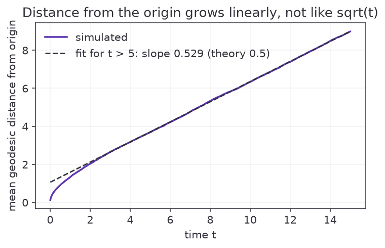
The line is offset above t / 2 rather than passing through the origin. That
is expected: coth(rho) exceeds 1 while rho is still small, so the particle
picks up extra distance early on before settling onto the asymptotic slope.
The rate is the slope, not the intercept.
Where they end up: the boundary circle
Because the motion is transient, the interesting limit is not a density on the disk but a point on the boundary circle. Every path converges almost surely to one, and the space of those limiting points is what is called the Poisson boundary.
The hyperbolic metric is rotationally symmetric about the origin, so for
particles started at the origin the limiting angle has to be uniform on
[0, 2 pi). ww.boundary_angle_histogram bins the angles of the particles
that have made it past a given Euclidean radius:
import numpy as np
import wanderwalk as ww

np.random.seed(0)
trajectory = ww.hyperbolic_simulator(T=1500, N=2000, dt=0.01)

counts, edges = ww.boundary_angle_histogram(
    trajectory[-1], radius_threshold=0.9, bins=12
)

print("counts:", counts)
print(f"{counts.sum()} of 2000 particles are past |x| = 0.9")
print(f"so {counts.sum() / 12:.2f} expected per bin")
counts: [180 158 176 155 157 170 169 150 151 148 165 156]
1935 of 2000 particles are past |x| = 0.9
so 161.25 expected per bin
Eyeballing a histogram is weak evidence. A chi-squared test is better, and
needs only SciPy from the notebooks extra:
import numpy as np
from scipy import stats
import wanderwalk as ww

np.random.seed(0)
trajectory = ww.hyperbolic_simulator(T=1500, N=2000, dt=0.01)
counts, _ = ww.boundary_angle_histogram(trajectory[-1], radius_threshold=0.9, bins=12)

chi2, p_value = stats.chisquare(counts)
print(f"chi-squared = {chi2:.4f}, p = {p_value:.4f}")
A p-value of 0.75 gives no reason to doubt uniformity, which is what the theory predicts.
boundary_angle_histogram can return nothing
If no particle has reached radius_threshold, the function returns
(None, None) rather than an empty histogram. Short runs, or a threshold
close to 1, will hit this. Check for it before unpacking if the run
length is not under your control.
Starting somewhere else
starting_point takes a point in the open unit disk. It is clamped just
inside the boundary if you hand it something on or past the rim, so the
conformal factor can never blow up:
import numpy as np
import wanderwalk as ww

disk = ww.PoincareDisk()

np.random.seed(0)
trajectory = ww.hyperbolic_simulator(T=200, N=100, dt=0.01, starting_point=[0.5, 0.5])

print("start was clamped to:", np.round(disk.project_to_manifold(np.array([0.5, 0.5])), 4))
mean_distance = disk.geodesic_distance_from_origin_multiple(trajectory[-1]).mean()
print(f"mean geodesic distance at t = 2: {mean_distance:.4f}")
[0.5, 0.5] has norm about 0.707, comfortably inside the disk, so nothing is
clamped. A starting point like [0.9, 0.9], with norm 1.27, would be pulled
back to just inside the boundary.
What next
- Density estimation, which covers
ww.disk_kdeand why it uses the exact hyperbolic distance rather than the Euclidean one. - The Poincare disk derivation, for the full derivation of the SDE from this project's conventions.