Brownian motion on the sphere

The unit sphere is the best surface to start with, because the long-run answer is known exactly. The sphere is compact and has constant positive curvature, so Brownian motion on it is recurrent, and the distribution of particles converges to the uniform distribution over the surface no matter where they started. That gives us something concrete to check the simulator against.

Everything on this page needs only the core install. The plots additionally use matplotlib, from the notebooks extra.

Running the simulation

import numpy as np
import wanderwalk as ww

np.random.seed(0)
trajectory = ww.sphere_simulator(T=200, N=500, dt=0.01, noise_type="isotropic")

print(trajectory.shape)

(200, 500, 3)

By default every particle starts at (1, 0, 0). Each step samples a random vector in the tangent plane at the particle's current position, scales it by the square root of dt, adds it, and then projects the result back onto the sphere. That projection is what keeps the particle exactly on the surface rather than drifting off it over thousands of steps.

Watching them spread

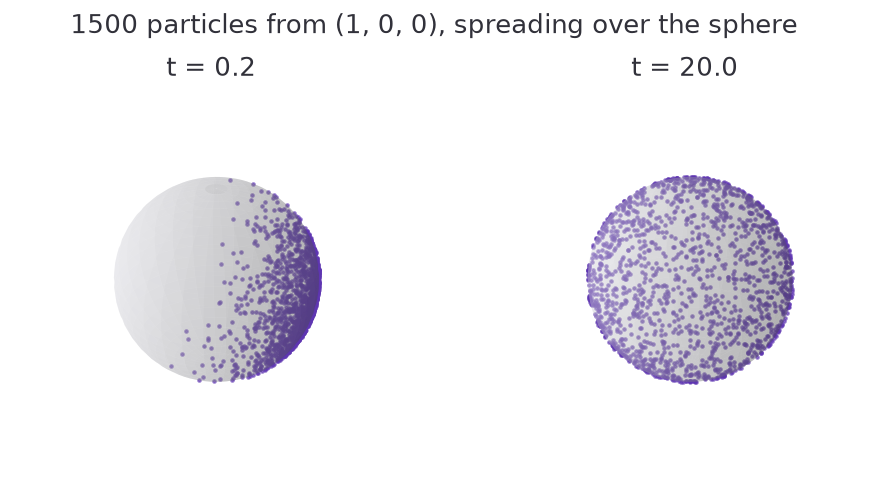
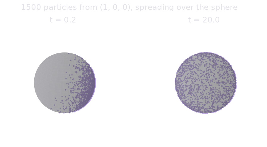
At t = 0.2 the particles are still a tight cap around the starting point. By t = 20 they cover the sphere. To draw that yourself:

import matplotlib.pyplot as plt
import numpy as np
import wanderwalk as ww

np.random.seed(0)
trajectory = ww.sphere_simulator(T=2000, N=1500, dt=0.01, noise_type="isotropic")
positions = trajectory[-1]

fig = plt.figure(figsize=(5, 5))
ax = fig.add_subplot(projection="3d")

u, v = np.mgrid[0:2 * np.pi:60j, 0:np.pi:30j]
ax.plot_surface(
    np.cos(u) * np.sin(v),
    np.sin(u) * np.sin(v),
    np.cos(v),
    color="lightgrey",
    alpha=0.3,
    linewidth=0,
)
ax.scatter(positions[:, 0], positions[:, 1], positions[:, 2], s=2, alpha=0.6)
ax.set_box_aspect([1, 1, 1])
ax.set_axis_off()
plt.show()

Checking convergence to uniform

The uniform distribution on the sphere is centered at the origin, so its mean position is the zero vector. The mean of our particles should therefore shrink toward zero as time goes on. That is a one-line diagnostic:

import numpy as np
import wanderwalk as ww

for T in (10, 100, 500, 2000):
    np.random.seed(0)
    trajectory = ww.sphere_simulator(T=T, N=2000, dt=0.01, noise_type="isotropic")
    center_of_mass = np.linalg.norm(trajectory[-1].mean(axis=0))
    print(f"t = {T * 0.01:6.1f}   |mean position| = {center_of_mass:.4f}")

t =    0.1   |mean position| = 0.9078
t =    1.0   |mean position| = 0.4243
t =    5.0   |mean position| = 0.0299
t =   20.0   |mean position| = 0.0386

It drops from 0.91 to about 0.03 and then stops improving. That floor is not a bug: with N particles the sample mean of a genuinely uniform distribution has magnitude on the order of 1 / sqrt(N), which for 2000 particles is about 0.022. Once the simulation reaches that scale, it is measuring sampling noise rather than any remaining structure.

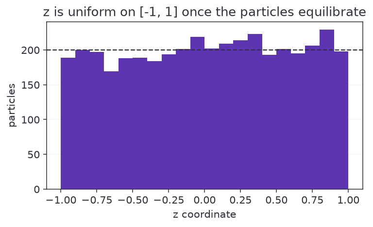
A sharper test: the z coordinate is uniform

Averaging positions is a blunt instrument. A much sharper check comes from a result of Archimedes: for a point distributed uniformly on the unit sphere, the z coordinate is uniform on [-1, 1]. Bands of equal height on the sphere have equal area, however close to the poles they sit.

import numpy as np
import wanderwalk as ww

np.random.seed(0)
trajectory = ww.sphere_simulator(T=2000, N=4000, dt=0.01, noise_type="isotropic")

counts, _ = np.histogram(trajectory[-1][:, 2], bins=5, range=(-1, 1))
print(counts, "expected 800 per bin")

[755 755 831 831 828] expected 800 per bin

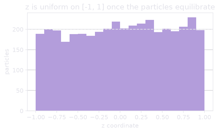
Five equal bands, roughly 800 particles each. The spread is consistent with counting noise, which is about sqrt(800), or 28 particles per bin.

Why this test is better

A distribution concentrated near the equator and one spread uniformly both have mean position zero, so the previous check cannot tell them apart. The z histogram can.

Anisotropic noise

Passing noise_type="anisotropic" constrains each particle to move along a single tangent direction rather than in all of them. On the sphere that direction is the tangential part of the fixed vector (1, 1, 1), which makes the motion one-dimensional. The particles cannot wander over the surface; they are stuck on the great circle through their starting point and the (1, 1, 1) axis.

That is a strong claim, and it is exactly checkable. Starting from (1, 0, 0), the plane containing the motion has normal (1, 0, 0) x (1, 1, 1), so every position must satisfy y = z:

import numpy as np
import wanderwalk as ww

np.random.seed(1)
trajectory = ww.sphere_simulator(T=400, N=1000, dt=0.01, noise_type="anisotropic")

print("largest |y - z| over all particles:", np.abs(trajectory[..., 1] - trajectory[..., 2]).max())

largest |y - z| over all particles: 0.0

Exactly zero, not merely small. The projection back onto the sphere is a rescaling, which cannot move a point out of a plane through the origin, so the constraint survives every step without any accumulated error.

This is a useful sanity check on the whole scheme: an anisotropic run that did not stay on its great circle would mean the tangent projection was leaking.

Choosing where to start

starting_point moves every particle to a different point. It is projected onto the sphere first, so you do not have to normalize it yourself:

import numpy as np
import wanderwalk as ww

np.random.seed(0)
trajectory = ww.sphere_simulator(
    T=50,
    N=100,
    dt=0.01,
    noise_type="isotropic",
    starting_point=[0, 0, 7],        # not a unit vector, and that is fine
)

print("first step, first particle:", np.round(trajectory[0, 0], 4))

first step, first particle: [0.1736 0.0394 0.984 ]

The particle begins at the north pole, because (0, 0, 7) is projected to (0, 0, 1) before the run starts.

What next

• The torus, where the surface is no longer symmetric and the particles do not spread evenly.
• Density estimation, for turning these final positions into a heatmap with ww.sphere_kde.
• The heat kernel, which compares the simulated distribution against the exact analytic answer rather than a summary statistic.